 Year  Jan  Feb  Mar Apr May  Jun  Jul   Aug   Sep  Oct  Nov  Dec
1 1869   NA   NA   NA  NA  NA   NA 2606  8885 10918 8699   NA   NA
2 1870   NA   NA 1146 682 545  540 3027 10304 10802 8288 5709 3576
3 1871 2606 1992 1485 933 731  760 2475  8960  9953 6571 3522 2419
4 1872 1672 1033  728 605 560  879 3121  8811 10532 7952 4976 3102
5 1873 2187 1851 1235 756 556 1392 2296  7093  8410 5675 3070 2049
6 1874 1340  847  664 516 466  964 3061 10790 11805 8064 4282 2904
** The original data consists of average monthly flow measurements from January 1869 to December 1984. Which I couldn't get access to the full dataset. For this exercise, I used Jan 1869 to December 1874.
From this mini data,
boxplot.py
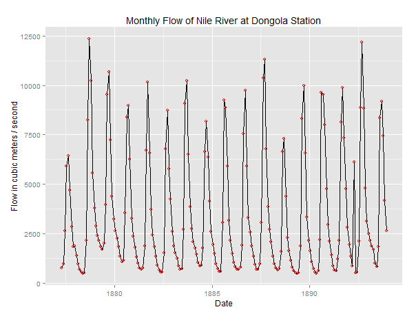
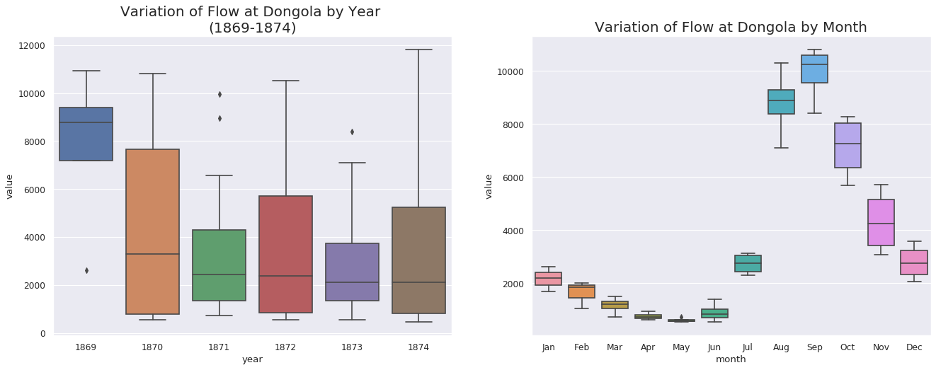
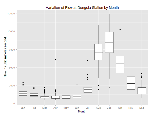
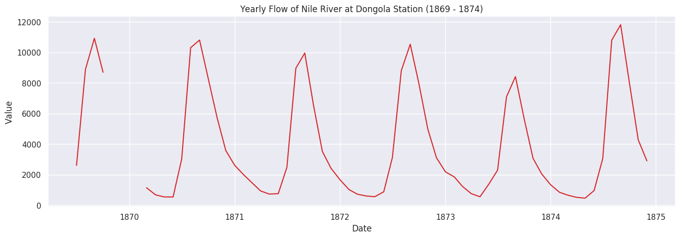
# Import Datadf = pd.read_csv('new_nile_format.csv', parse_dates=['date'], index_col='date')df.reset_index(inplace=True)#print(df)# Prepare datadf['year']= [d.year for d in df.date]df['month']= [d.strftime('%b')for d in df.date]years = df['year'].unique()x = df['year'].valuesy1 = df.date# Draw Plotfig, axes = plt.subplots(1, 2, figsize=(20,7), dpi=80)sns.boxplot(x='year', y='value', data=df, ax=axes[0])sns.boxplot(x='month', y='value', data=df.loc[~df.year.isin([1869, 1874]), :])# Set Titleaxes[0].set_title('Variation of Flow at Dongola by Year \n(1869-1874)', fontsize=18); axes[1].set_title('Variation of Flow at Dongola by Month', fontsize=18)plt.show()defplot_df(df,x,y,title="",xlabel='Date',ylabel='Value',dpi=100): plt.figure(figsize=(16,5), dpi=dpi) plt.plot(x, y, color='tab:red') plt.gca().set(title=title, xlabel=xlabel, ylabel=ylabel) plt.show()plot_df(df, x=df.date, y=df.value, title='Monthly Flow of Nile River at Dongola Station (1869 - 1874)')
From the website: Long Memory and the Nile: Herodotus, Hurst and H. We can see that there is a similarity between variation of flow at Dongola Station by Month and Monthly Flow of Nile River Dongola Station.
Limitation:
** The original data consists of average monthly flow measurements from January 1869 to December 1984. Which I couldn't get access to the full dataset. For this exercise, I used Jan 1869 to December 1874.
Hurst Exponent
The goal of the Hurst Exponent is to provide us with a scalar value that will help us to identify (within the limits of statistical estimation) whether a series is mean reverting, random walking or trending.
The idea behind the Hurst Exponent calculation is that we can use the variance of a log price series to assess the rate of diffusive behavior. For an arbitrary time lag ττ, the variance is given by:
Since we are comparing the rate of diffusion to that of a Geometric Brownian Motion, we can use the fact that at large ττ we have that the variance is proportional to ττ in the case of a GBM:
⟨∣log(t+τ)−log(t)∣2⟩∼τ⟨∣log(t+τ)−log(t)∣2⟩∼τ
The key insight is that if any autocorrelations exist (i.e. any sequential price movements possess non-zero correlation) then the above relationship is not valid. Instead, it can be modified to include an exponent value "2H2H", which gives us the Hurst Exponent value HH:
⟨∣log(t+τ)−log(t)∣2⟩∼τ2
A time series can then be characterized in the following manner:
H<0.5H<0.5 - The time series is mean reverting
H=0.5H=0.5 - The time series is a Geometric Brownian Motion
H>0.5H>0.5 - The time series is trending
In addition to characterization of the time series the Hurst Exponent also describes the extent to which a series behaves in the manner categorized. For instance, a value of HH near 0 is a highly mean reverting series, while for HH near 1 the series is strongly trending.
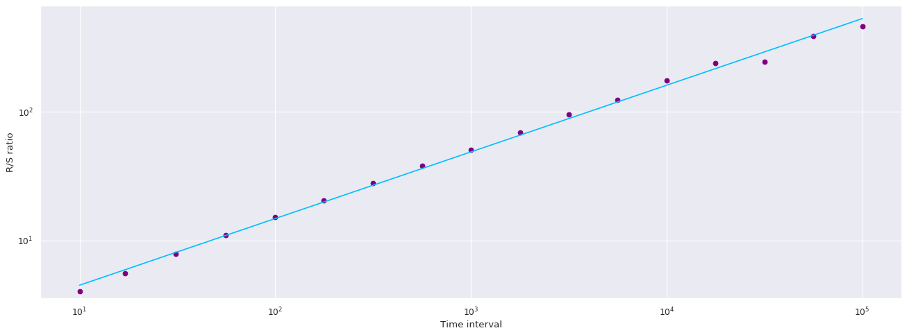
The code below represents the hurst exponent and random changes value. Due to its small sample data size. I wasn't able to produce a hurst exponent. Instead, I've substitute with a random series.
hurst.py
from hurst import compute_Hc, random_walk# series = random_walk(99999, cumprod=True)np.random.seed(42)random_changes =1.+ np.random.randn(99999)/1000.nile_series = df.value.cumprod#larger_nile_series = nile_series + 25.print(random_changes)print(df.value.cumprod)#Series length must be greater or equal to 100, Currently 72 due to the small size of the data.series = np.cumprod(random_changes)# change the variable with nile_series#Setting up Hurst exponent#print(df.value.len())print(df.value.std())print(df.value.mean())#print(df.value.cummax())#print(df.value.cummin())#print(df.value.cumprod())# Evaluate Hurst equationH, c, data =compute_Hc(series, kind='price', simplified=True)# Plotf, ax = plt.subplots(figsize=(20,7), dpi=80)ax.plot(data[0], c*data[0]**H, color="deepskyblue")ax.scatter(data[0], data[1], color="purple")ax.set_xscale('log')ax.set_yscale('log')ax.set_xlabel('Time interval')ax.set_ylabel('R/S ratio')ax.grid(True)plt.show()print("H={:.4f}, c={:.4f}".format(H,c))
Any questions or concerns, you can email me here: steven.yoo@nyu.edu